Distillation becomes a computable budget problem

Consider the scale of the evidence. This study, accepted at ICML 2025, covers models ranging from roughly 143 million to 12.6 billion parameters, with up to 512 billion training tokens. The authors fit their formula using 73 supervised training runs and 697 distillation runs.

In supervised training, the student updates its parameters based on the correct next token. In distillation, the student learns to imitate the teacher's probability distribution over the entire vocabulary. The true answer only tells the student which token is right; the teacher's distribution also reveals how plausible each of the other candidates is. That extra information is often called soft labels.

Previous distillation experiments typically fixed a single teacher and then compared different students. That approach can answer whether a given teacher helps, but not how strong the teacher should be, how large the student should be, or whether the same compute would be better spent directly on the student. This paper varies the teacher's size, the teacher's training tokens, the student's size, and the student's training tokens all at once, mapping all four variables onto a single landscape.

The key finding is that, within the experimental range, the influence of teacher size and teacher training data on the student can be compressed into a single variable: the teacher's cross-entropy loss. Intuitively, cross-entropy reflects how much probability the model assigns to the correct next token; lower is generally better. This reduces the prediction of student loss to three core inputs: teacher loss, student parameter count, and the number of tokens the student has seen.

That simplification is significant. Engineering teams do not need a separate empirical rule for every teacher architecture. As long as the teacher remains within the paper's tested same-data-distribution Transformer setting, its size and training volume can be summarized by a single quality measure: teacher loss. But reducing teacher quality to teacher loss is an empirical simplification from these experiments, not a universal result across architectures, datasets, or distillation methods.

The resulting map leads to three testable conclusions: student loss depends jointly on teacher loss, student capacity, and student training tokens; fixing the student reveals a capacity gap where an overly strong teacher hurts performance; and the advantage of distillation over supervised training is constrained both by a student data threshold and by whether the teacher can be reused. The latter two are verified by a U-shaped curve for fixed students and four different cost accounting methods.

Student loss depends on teacher quality, student capacity, and training data

The formula first fits a supervised baseline—larger models with more data achieve lower loss—then adds terms for teacher quality and a capacity inflection. You don't need to memorize the coefficients; just understand the three directions:

1. A larger student can express more patterns, so loss generally decreases.
2. More tokens let the student fit the teacher more closely, so loss generally decreases.
3. As the teacher goes from weak to strong, the student initially benefits; but beyond a certain matching point, further improvement in the teacher can hurt the student.

These directions are supported by three layers of experimental design. The first is the supervised baseline: the authors use both fixed model sizes with varying data and IsoFLOP curves, where model size and token count are varied together under a constant FLOPs budget. Looking only at optimal models for each compute budget would make the token-to-parameter ratio roughly fixed, preventing the model scale term from being separated from the data term.

The second layer is the training objective. Supervised training uses one-hot labels—1 for the correct token, 0 for all others. Distillation applies a softmax to the teacher's raw scores, turning them into a probability distribution over the whole vocabulary that sums to 1, and the student learns that distribution. For a fixed teacher, this cross-entropy is equivalent to forward KL divergence, measuring the KL divergence from the teacher distribution to the student distribution, since the teacher's own entropy is constant.

The third layer is the distillation experiment itself: fixing the teacher and moving the student along multiple IsoFLOP curves isolates the student size and data terms; fixing the student and moving the teacher along multiple IsoFLOP curves tests whether teacher size and teacher tokens can be captured by teacher loss alone; and broad teacher-student pairings at fixed token-to-parameter ratios reveal the full capacity gap. These three protocols together support the formula rather than relying on a single curve.

Figure 5. The top panel compares predicted values against measured ones; the bottom shows relative error. The authors report a relative prediction error of about 1% for the main fit.

This law isn't derived from first principles; it's an empirical function that fits very well within the given experimental domain. Its value is to turn the relationship between teacher, student, and data—previously something you had to figure out through trial and error—into something that can be fitted, compared, and used for compute-budget optimization. It doesn't claim to provide permanent coefficients for all models.

A stronger teacher can make the student worse

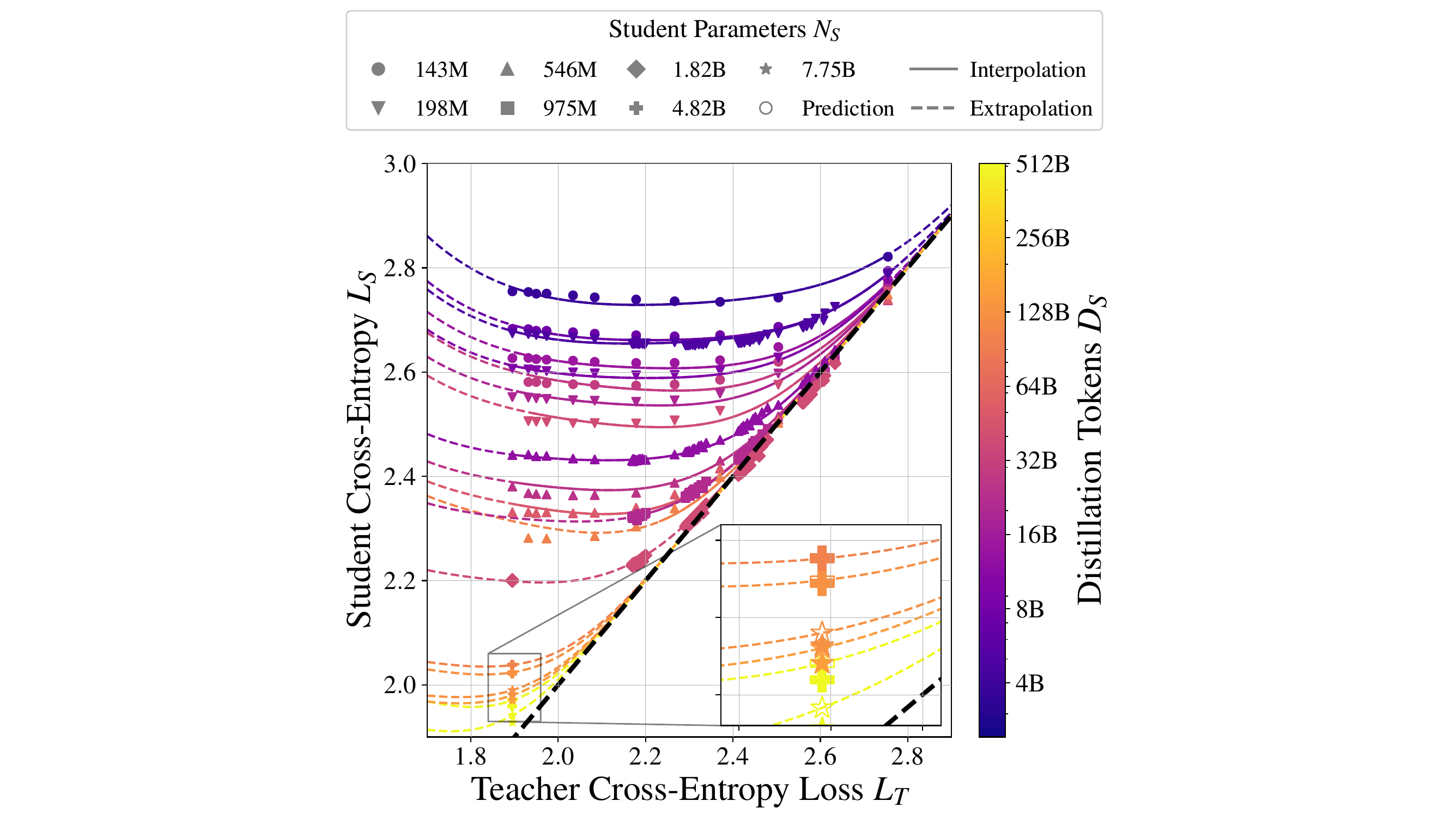
The capacity gap overturns the idea that a stronger teacher is always better. With a fixed student size and training data, as teacher loss decreases from high to low, student loss first drops and then rises, forming a U-shaped curve. A teacher that's too weak doesn't provide enough information; a teacher that's too strong can also be harder for the student to learn from.

Take the interaction above, which uses the fitted coefficients from Table 6 of the paper. It fixes a student with about 198 million parameters and training tokens roughly 20 times its parameter count. As you adjust teacher loss, the predicted student loss bottoms out near a teacher loss of about 1.9 nats (nats are the unit of cross-entropy measured with natural logarithms). If the teacher gets stronger and its loss drops to 1.6, the predicted student loss actually rises from about 2.53 to 2.61. These numbers are just illustrative examples within the fitted range of the paper, not universal thresholds for other models.

The authors propose a theoretical explanation: misaligned expressive capacity. A larger teacher continues to learn complex patterns that the student simply cannot represent. To fit those patterns, the teacher may reallocate probability mass, reducing emphasis on patterns the student could have learned. The student is trying to approximate the teacher's full distribution with limited capacity, so a teacher that is closer to the true distribution isn't necessarily easier for that student to imitate.

The paper tests this mechanism with two simplified models. Kernel regression provides an analytically tractable example: when the teacher devotes more representational power to basis functions outside the student's hypothesis space, the student's error provably increases. A synthetic multilayer perceptron experiment then reproduces the same U-shaped phenomenon: student performance turns for the worse when the teacher starts to capture basis functions that are unreachable by the student. Together these support the idea of capacity mismatch, though they don't constitute a causal proof of the internal mechanics of large Transformers.

Calibration experiments rule out an overly simple explanation. A student that learns the teacher's full distribution remains largely calibrated on real data, while a student that only learns the teacher's top-1 prediction is noticeably overconfident. Conversely, when judged against the teacher's top-1 as ground truth, the top-1 student appears better calibrated, and the full-distribution student might seem underconfident. This shows that matching the teacher's answer and matching the teacher's uncertainty are two different tasks. The authors also observe that when the teacher is stronger, students find it harder to replicate the full distribution in regions where the teacher has low confidence. This aligns with the capacity gap, but the binned calibration plots only offer clues; they don't alone prove causation.

This changes the teacher selection rule. The goal isn't to find the teacher with the lowest loss, but to find a teacher matched to a given student and data budget. As the student grows or sees more data, that matching point shifts; a teacher that was originally too strong can become useful again.

Whether distillation is worth it depends on amortizing teacher cost

The same scaling law gives completely different recommendations depending on how you account for costs. Tables 2 and 5 in the paper compare four distinct scenarios. Total cost is broken into three parts: student training, which is roughly three times the student's per-token forward FLOPs multiplied by the number of student tokens; teacher logit generation, which is the teacher's forward FLOPs multiplied by the number of student tokens; and teacher pretraining, which is three times the teacher's per-token forward FLOPs multiplied by teacher tokens. The four scenarios simply decide whether to include the latter two terms; they aren't claiming real teachers are actually free.

The first scenario is full teacher amortization: the teacher already exists and logits are freely available, so the budget only counts student updates. This is the most favorable setting for distillation. When the student's training data is limited, the teacher distribution provides more information than individual real tokens, so distillation can achieve lower loss with less student compute. But as data keeps increasing, supervised training catches up; with enough data and compute, supervised training can match or exceed distillation.

The second scenario assumes the teacher is already trained, but every student token requires one forward pass through the teacher. Distillation can still have an advantage, but the larger the teacher, the more expensive it is to generate soft labels, so the optimal teacher doesn't grow without bound.

The third scenario counts teacher pretraining but not teacher inference: the teacher needs to be trained from scratch, but the generated logits are stored and can be reused across training restarts or across multiple students. This accounts for the one-time teacher cost while spreading the per-token inference cost thin. It suits scenarios where soft labels are cached or where multiple students are trained in batches.

The fourth scenario is closest to "training a teacher specifically for one student": all three costs are included—teacher pretraining, teacher forward passes over student data, and student training. In this least favorable case, the paper finds that supervised training is usually better. The reason isn't mysterious: you spend a lot of compute to get the teacher, then have the teacher read all the student data, and finally the student completes its own training. The data efficiency gains from soft labels often don't outweigh those two added costs.

Figure 1. The surface shows how teacher loss and student size relate to student loss; the fixed slice on the right reveals the capacity gap.

The paper also draws a more nuanced conclusion: the benefit of weak-to-strong distillation is primarily a finite-data phenomenon. When the student has only seen a small amount of data, the teacher distribution offers a denser learning signal; as distillation data becomes plentiful, the student approaches the teacher rather than unconditionally surpassing it. The idea of a "weak teacher producing a strong student" doesn't hold up independently of data volume and evaluation criteria.

This also clarifies an apparent conflict with "patient teacher" studies. In that line of work, "patient" means letting the student learn over more distillation tokens—i.e., a longer student training run—not continuing to pretrain the same teacher. This paper also observes that more distillation improves the student, but when compared against a supervised baseline using real tokens on the same C4 distribution, continued distillation can eventually become compute-suboptimal. Earlier studies used different data distributions and different supervised baselines. Appendix E.6 gives a stricter bound: when you pick the optimal teacher for each student size, the lower bound on student cross-entropy with infinite distillation data matches the lower bound from supervised training.

The fixed-token and fixed-compute profiles also show that the advantage region isn't a static boundary: larger students and higher budgets can typically absorb stronger matched teachers, but when you keep the student fixed and keep adding data, the relative advantage of distillation over supervised training shrinks. The authors use SLSQP, a numerical optimization method that searches for the lowest-loss combination under a total compute constraint, to find the optimal teacher, teacher training volume, and student tokens under each of the four cost settings—rather than using a single teacher across all budgets.

Downstream evaluations in the appendix add a practical caveat to these budget conclusions: if task scores improve with cross-entropy, the four accounting methods remain informative; but if a model is near random on a task, the cross-entropy optimum calculated from the formula doesn't replace actual capability verification. The paper also lists two-sided implications: more reliable scaling laws could reduce trial-and-error and lower the inference cost of small models over their lifecycle, but biases from teacher pretraining can be passed on to students, and stronger, cheaper small models also lower the barrier to misuse. These are deployment risks that don't change the law itself but do shift the product-level answer to whether distillation is worth doing.

So when deciding whether distillation is cost-effective, ask three questions: Does the teacher already exist? How many students or training runs will it serve? Is the current student still in the data-scarce regime? When a teacher can be reused across multiple students, sizes, or deployment targets, the pretraining cost is amortized and the economics of distillation improve significantly. If it only serves one student, don't let "faster student training" hide the teacher's cost.

The paper's training recipe: temperature 1 and top-k 128

If your task closely matches the paper's setup—same text distribution, token-level prediction, student imitating the teacher's full probability distribution—the appendix offers a set of recipe parameters that work as a starting point for initial experiments.

The formula's coefficients weren't eyeballed from a few curves. The authors fit 73 supervised and 697 distillation samples in log space using a Huber loss, which reduces the influence of a few large residuals; they then searched from multiple starting points to reduce the risk of landing in a local optimum. This methodology, together with Figure 5's roughly 1% relative error, forms the statistical foundation for the recipe's numbers.

Regarding soft label weights, pure distillation—where the student learns only from the teacher's distribution—proved robust across most experiments. Mixing in a small amount of true token loss didn't hurt, but as long as the distillation weight stayed above 0.5, results were largely flat. Temperature controls how smooth the teacher's probability distribution is: higher temperatures give more weight to low-probability candidates. In the authors' tests, a temperature of 1 worked best. For optimization, µP is a parameterization method that helps hyperparameters like learning rate transfer across model scales. The paper found that a learning rate of 0.01 under simplified µP transferred cleanly across the tested sizes.

Storage is the most practical obstacle to full-distribution distillation. At each training position, the teacher outputs one raw score for every vocabulary token; these scores, called logits, are then converted into probabilities. The paper estimates that saving float32 full-vocabulary logits for C4's roughly 2 trillion tokens would require about 260 PB. To work around this, the authors tested keeping only the top-k tokens by teacher probability, combined with a fraction of true label loss. With top-k at 128 and a distillation weight of 0.7, the student's loss came within 0.01 nats of full-distribution distillation. That suggests the cache can be cut dramatically—but 128 is not some universal constant that works across vocabularies and tasks. You'll need to re-test it on your own distribution.

The authors also compared two directions for computing distribution divergence. Forward KL measures the difference from the teacher's distribution to the student's, while reverse KL flips the order. In the paper's experiments, forward KL achieved a loss of 2.42 versus 2.70 for reverse KL, making forward KL the better choice. That said, all these numbers come from one fixed training stack and are best treated as a starting point rather than a default standard.

FLOPs estimates also should not be transferred mechanically from the common heuristics of about 2N FLOPs per token for a forward pass and about 6ND FLOPs to train on D tokens. Since the paper focuses on small models with a 4096-token context, attention and vocabulary projection cannot be dismissed. For a fixed width-to-depth ratio, the authors express forward FLOPs as a sum of three terms: a parameter-dominated term proportional to N, a context-dependent term proportional to N raised to the two-thirds power, and a vocabulary-related term proportional to N raised to the one-third power. The appendix breaks down attention, MLP, normalization, vocabulary projection, and backward pass item by item, comparing approximations against configuration tables. For example, a 143M non-embedding parameter model, if estimated using only 2N, would have its cost underestimated by about 36%; adding the context and vocabulary terms brings the error down to roughly 0.34%. For small-model, long-context budgets, the FLOPs definition itself can change which route is optimal.

This scaling law does not directly apply to reasoning traces or cross-distribution distillation

The paper studies Transformers trained on C4 English, where teacher and student share the same data distribution, use 4096-token sequences, and the distillation target is the teacher's full per-token probability distribution. What it doesn't cover: training on whole teacher-generated answers, using only hard labels, learning chain-of-thought, cross-lingual transfer, cross-domain data, or settings where teacher and student use different tokenizers.

The experimental setup is similarly uniform: multi-head attention, Pre-Norm with RMSNorm, RoPE positional encoding, fixed width-to-depth ratio, and fixed feedforward ratio—all trained in AXLearn. Teacher and student are trained on different slices of C4 English. C4 contains roughly 180 billion tokens, with about 90 billion non-repeated training tokens allocated to each of the teacher and student; training beyond that means reusing data. The authors cite prior work on repeated data, which shows that in C4 supervised training, repeating data up to about four times has minimal impact on loss. They also acknowledge explicitly that they cannot confirm whether this still holds for distillation, and that it shouldn't replace validation across datasets.

To see where these findings sit in the research landscape, related work and author contributions can be compressed into three layers:

• Problem lineage: Classic knowledge distillation, self-distillation, patient teachers, capacity gaps, calibration, and weak-to-strong generalization research each ask distinct questions: what students learn, how long they learn, whether the teacher might be too strong, and whether the probabilities are trustworthy.
• Method scaffold: Supervised scaling laws, C4 and repeated data, SLSQP, Huber, µP, attention and tensor programs, Transformer training, and FLOPs estimation support comparison baselines, robust fitting, cross-scale parameter transfer, and cost calculations. LLaMA, Gemma, transfer learning, downstream evaluation, and inference compute provide practical context or future directions rather than validated objects of study.
• Evidence division: The author contributions table assigns training and IsoFLOP design, formula fitting, kernel regression and synthetic MLP, calibration, and Top-k/KL analysis to specific members. The formulas are therefore backed by three kinds of support—experimental, theoretical examples, and engineering validation—rather than being isolated curve fits.

The boundaries of downstream capability also need to be acknowledged. The authors found that some standard English tasks align with cross-entropy trends, but their models perform near chance on GSM8K and MMLU. The paper therefore does not demonstrate that a 0.01 drop in cross-entropy translates into proportional gains in reasoning or knowledge QA. And it doesn't offer off-the-shelf scaling coefficients for the kind of reasoning-trace distillation popularized by DeepSeek-R1.

Three decision frameworks do transfer: pick a teacher matched to the student rather than the strongest available; include student training data thresholds in comparisons instead of single-shot accuracy; and account for the full teacher training and inference costs, spread explicitly across however many students share them.

The specific coefficients, however, need to be re-fit. Any change in data distribution, model architecture, loss objective, vocabulary, sequence length, or training recipe can shift the capacity gap and the compute optimum. Treating the paper as a budget-modeling methodology is genuinely useful. Lifting numbers straight from Table 6 and applying them to another model project yields answers that look precise but have no evidentiary basis.

The bottom line: distillation's advantage comes from the extra information in the teacher's distribution, but that information only translates into real compute savings when the student can absorb it, the data is insufficient on its own, and the teacher's cost can be amortized.