Google Research releases TimesFM-3, a time-series foundation model that forecasts what comes next
It doesn't predict abstract events. Instead, it outputs concrete numbers shaped by multiple time curves and known future plans: sales, traffic, load, prices, and the uncertainty around all of them.
- TimesFM-3 packs 330 million parameters and was trained on over one trillion time points. It natively handles multiple targets, historical covariates, and future-known covariates.
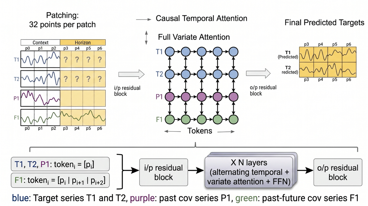
- The model arranges time and variables into a 2D grid, alternating information exchange along both axes. A single forward pass produces the entire forecast horizon plus nine quantiles.
- Google reports the model ranks first on average across point and probabilistic forecasting benchmarks including GIFT-Eval, FEV-Bench, and TIME. But a leading average doesn't replace a proper business backtest.
- Code is open, but the default 3.0 pretrained weights are currently restricted to non-commercial, non-production use.
Google Research has released TimesFM-3, a time series foundation model. This is the first version of the TimesFM series built natively for multivariate forecasting: the model can simultaneously predict multiple interacting time series, and can also incorporate external information such as foot traffic, weather, promotions, and holidays into its predictions.
In theory, this means it can predict the future—specifically, future values of time-varying quantities like sales, foot traffic, equipment load, and prices. This is not about forecasting open-ended events. The real question is whether a general-purpose model, without task-specific fine-tuning, can handle situations where outcomes depend on multiple co-varying curves and known future plans. TimesFM-3's answer is to organize time and variables into a two-dimensional grid, exchanging information alternately along both axes.
1. Moving beyond univariate limits to true multivariate forecasting
The previous pain point: The TimesFM-2.5 base model primarily forecasted the future of a single target series based on its own history. Real-world prediction, however, rarely depends on just one curve. Forecasting next month's ice cream sales, for instance, requires more than just past sales data; you also need to consider cone and syrup sales, historical customer traffic, weather forecasts, promotion schedules, and holidays.
TimesFM-2.5 could later incorporate covariates through XReg. But that differs from TimesFM-3's native multivariate capability. The former adds external regressors to a univariate base model, while the latter learns the joint dynamics of multiple target series and covariates from the pretraining phase onward.
The current capability: TimesFM-3 has 330 million parameters and was pretrained on over 1 trillion real and synthetic time points. It supports zero-shot forecasting—no task-specific fine-tuning is required. The model can directly accept three types of input:
- Multiple targets: Simultaneously predict multiple interacting time series, such as sales for different brands, stores, or product categories.
- Historical covariates: Information known only in the past, such as historical foot traffic and equipment status.
- Future-known covariates: Information that extends from history into the prediction period, such as scheduled promotions, holidays, and currently available weather forecasts.
"Future-known" doesn't mean clairvoyance. Holidays and promotion schedules can be set in advance, but weather forecasts carry inherent uncertainty; the model uses information that was available at the time of prediction. Zero-shot also means you don't need to retrain the model for each specific store, device, or business series—but data cleaning, variable selection, time alignment, and backtesting are still on you.
2. Organizing time and variables into a two-dimensional grid
Multivariate analysis isn't just about concatenating columns of data. Feeding every individual time point into a Transformer becomes computationally expensive as sequences grow longer. TimesFM-3 follows the established TimesFM approach: it groups 32 consecutive time points into a patch and encodes each patch as a token. Series with different units are also normalized separately, preventing a sales figure in hundreds of dollars from overwhelming a switch variable ranging from 0 to 1 just because of scale.
Each token corresponds to a standard patch for target series and covariates known only in the past. Future-known covariates get an extra "look-ahead" step: the current patch is concatenated with its future patches. This way, when the model processes a specific time position, it can already see scheduled promotions or holidays within the forecast horizon.

Inside the main architecture, attention alternates between two directions.
- Along the time axis, each series only attends to its own past. This is causal attention—it captures trends, seasonality, and prior changes while preventing the target series from peeking at future actuals.
- Along the variable axis, each time position can attend to other series. Ice cream sales can reference cone sales, store sales can reference foot traffic, and target series can read covariates like promotions and weather.
The horizontal pass handles "how has this curve evolved," while the vertical pass handles "what's happening in other curves at the same time." After multiple alternating layers, the model has learned not just a set of independent series, but a set of relationships that evolve together over time.
This also explains why multivariate modes can outperform univariate ones: gains come from additional information and cross-series relationships. If the series aren't stably correlated, or if future covariates are unreliable, feeding in more variables won't automatically help.
3. Generating the entire forecast horizon in a single forward pass
Previous versions of TimesFM predicted one patch, then fed that result back into the input to predict the next patch. Longer forecast horizons meant more iterations, leading to higher latency and compute costs. Errors from earlier steps could also cascade into subsequent predictions.
TimesFM-3 borrows the idea of continuous patch masking, placing the entire forecast horizon into the model from the start:
- Future target values and covariates known only in the past use mask placeholders, since their future values are unknown.
- Future-known covariates, such as holidays and promotion plans, remain visible.
- Time attention and variable attention process both the history and forecast regions simultaneously on the same grid.
- The model fills in the results for all target series across the entire forecast horizon in one step.
The official PyTorch implementation will pad the user-requested forecast length up to an integer multiple of the output patch size, call model.decode() once, and then trim the extra positions. This "single pass" refers to the model's forward process; it doesn't mean compute is independent of forecast length. A longer horizon still means more tokens are fed into that same forward pass.
The output isn't just a single confident-looking curve. For each target and each future time point, TimesFM-3 produces quantiles ranging from the 10th to the 90th percentile, for 9 quantiles in total. The median serves as a point forecast, while the lower and higher quantiles form a set of uncertainty bands. Distant horizons or less stable signals typically result in wider intervals.
4. Bringing known future plans into the forecast
Google demonstrated this mechanism with a synthetic ice cream sales example. The red line represents a univariate forecast based only on historical sales, which mainly continues the weekly pattern. The blue line additionally incorporates future promotion days, leading to higher sales predictions on scheduled promotion dates.
Toggle input conditions and watch how the curve responds over the same forecast window.
Mechanism demo: curves use standardized illustrative values; TimesFM-3 is not invoked, and no real business forecasts are generated.

Illustrative synthetic case: roughly 20% reflects the relationship in the example, not a general lift for real promotions.
In the training data, the example established a relationship where promotions drive roughly a 20% lift in sales. The multivariate mode learns this relationship from historical promotion days and sales moving together, then applies it to future scheduled promotions. Over the course of the month, the blue line aligns more closely with the revenue logic of the case than the red line that ignores the promotion schedule.
This chart demonstrates that the model can use future covariates to recover a relationship that already exists in its context. It does not prove promotions universally drive 20% growth in reality, nor does it resolve the causal question of whether promotions actually cause sales increases. Real-world business involves discount levels, inventory, competitive actions, and changes in promotion targets.
5. Three benchmarks confirm the multivariate capability works
Google compared TimesFM-3 against other time series foundation models—including TimesFM-2.5, Chronos-2, Toto 2.0, and TiRex—on GIFT-Eval, FEV-Bench, and TIME. The horizontal axis measures average rank on point forecasting tasks; the vertical axis measures average rank on probabilistic forecasting tasks. Lower is better on both, so models closer to the bottom-left corner have better combined rankings.
X-axis = average rank for point forecasts; Y-axis = average rank for probabilistic forecasts; lower-left is better.


Average rank reflects overall position across the included tasks and model sets, not a win on every dataset or business metric.
All three charts tell the same story: TimesFM-3's multivariate mode sits at the bottom-left. When all inter-variable information and covariates are disabled and it's used purely as a univariate model, its average rank still matches or improves upon the other reproducible foundation models in the charts. Enabling multivariate mode further improves its standing.
These results carry two important implications. First, the model didn't trade univariate performance for multivariate capability: it still works as a general-purpose forecasting model without covariates. Second, additional variables provide consistent average gains across multiple tasks—this isn't just a phenomenon in the promotion example.
Average rankings, however, can mask individual differences. They show the model's overall position across tasks, but don't guarantee it wins on every dataset, and they don't account for any company's specific loss functions, inventory constraints, or error costs. The comparison reflects the set of models included at release time. Custom models trained on proprietary business data, classic statistical models, or later models would need to be re-evaluated in the same backtesting framework.
6. Predicting the future isn't the same as being ready for production
TimesFM-3 is available via GitHub code and Hugging Face weights. The official interface takes a target array shaped as "variables × history length"; future-known covariates should cover "history length + prediction length". The output includes both point forecasts and 9 quantiles for each target series.
Before experimenting, make sure of four things:
- Data is aligned to the same time frequency, and missing values, outliers, and generation timestamps for future covariates are handled properly.
- Covariates are actually available at the time of prediction—don't pretend that data known only in hindsight is future-known information.
- The errors, inventory costs, or risk metrics that matter to your business are better than the current baseline in rolling backtests.
- Input size fits the current implementation. The official code supports a maximum history length of 15,360 time points; the benchmark evaluator handles at most 32 variables in a single forward pass, with more targets processed in chunks, and excessive covariates potentially downsampled.
Licensing is a harder boundary. The repository code is Apache-2.0, but the default pretrained weights for TimesFM 3.0 currently use a separate non-commercial license, limiting use to non-commercial, non-production purposes. Downloading weights for research validation is fine; integrating them into a paid product or production forecasting system is not within the license's scope.
Google says BigQuery integration for TimesFM-3 will arrive in the coming weeks. For now, AI.FORECAST remains the immediately usable option, but it still runs on TimesFM-2.5's univariate capabilities. So TimesFM-3 is best suited for local research and business backtesting right now; "code and weights are public" shouldn't be mistaken for "enterprises can deploy immediately without restrictions."
TimesFM-3 advances multivariate forecasting from "build a custom model for every business" to "run a general-purpose model for initial backtests." It lowers the barrier to experimentation, but also places new responsibility on the user: figuring out which variables are truly available at prediction time, whether cross-series relationships will persist, and whether average benchmark gains translate into real business improvements. The model brings more real-world information into the forecast, but the final judgment still needs to happen on your own data.
Members can copy or download the full Markdown, and let their AI subscribe and ask.
Found this useful? Leave your email — every new explainer, the moment it's out. Unsubscribe anytime.